💾Praktikum 1

Klasifikasi Iris dengan Perceptron

Deskripsi

Pada pratikum ini, Anda diminta untuk melakukan klasifikasi bunga iris dengan menggunakan model Perceptron. Anda dapat menggunakan dataset iris pada praktikum sebelumnya.

Untuk nembah pemahaman Anda terkait dengan model Perceptron, pada pratkikum ini Anda akan membuat model Perceptron tanpa menggunakan library.

Langkah 1 - Import Library

import numpy as np
import matplotlib.pyplot as plt
import pandas as pd
import seaborn as sns

Langkah 2 - Load Data dan Visualisasi

df = pd.read_csv('iris.csv', header=None)
setosa = df[df[4] == 'Iris-setosa']
versicolor = df[df[4] == 'Iris-versicolor']
virginica = df[df[4] == 'Iris-virginica']

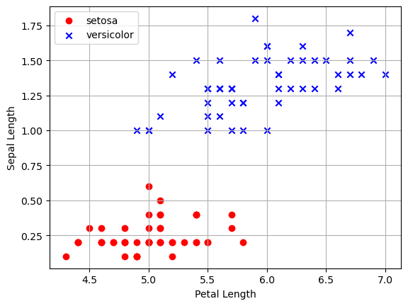
a, b = 0, 3
plt.scatter(setosa[a], setosa[b], color='red', marker='o', label='setosa')
plt.scatter(versicolor[a], versicolor[b], color='blue', marker='x', label='versicolor')

plt.xlabel('Petal Length')
plt.ylabel('Sepal Length')
plt.legend(loc='upper left')
plt.grid()
plt.show()

Hasil visualisasi,

Langkah 3 - Membuat Kelas Perceptron

class Perceptron(object):
    def __init__(self, eta=0.01, n_iter=10):
        self.eta = eta
        self.n_iter = n_iter
    
    def fit(self, X, y):
        
        self.w_ = np.zeros(1 + X.shape[1])
        self.errors_ = []
        
        for _ in range(self.n_iter):
            errors = 0
            for xi, target in zip(X, y):
                update = self.eta * (target - self.predict(xi))
                self.w_[0] += update
                self.w_[1:] += update * xi
                errors += int(update != 0.0)
            self.errors_.append(errors)
        return self
    
    def net_input(self, X):
        return np.dot(X, self.w_[1:]) + self.w_[0]
    
    def predict(self, X):
        return np.where(self.net_input(X) >= 0.0, 1, -1)

Langkah 4 - Pilih Data dan Encoding Label

y = df.iloc[0:100, 4].values # pilih 100 data awal
y = np.where(y == 'Iris-setosa', -1, 1) # ganti coding label
X = df.iloc[0:100, [0, 3]].values # slice data latih

Langkah 5 - Fitting Model

ppn = Perceptron(eta=0.1, n_iter=10)
ppn.fit(X, y)

Langkah 6 - Visualisasi Nilai Error Per Epoch

plt.plot(range(1, len(ppn.errors_)+1), ppn.errors_)
plt.xlabel('Epochs')
plt.ylabel('Number of updates')
plt.show()

Hasil visualisasi,

Langkah 7 - Visualiasasi Decision Boundary

# buat fungsi untuk plot decision region

from matplotlib.colors import ListedColormap

def plot_decision_regions(X, y, classifier, resolution=0.02):
    # setup marker generator and color map
    markers = ('s', 'x', 'o', '^', 'v')
    colors = ('r', 'b', 'g', 'k', 'grey')
    cmap = ListedColormap(colors[:len(np.unique(y))])
    
    # plot the decision regions by creating a pair of grid arrays xx1 and xx2 via meshgrid function in Numpy
    x1_min, x1_max = X[:, 0].min() - 1, X[:, 0].max() + 1
    x2_min, x2_max = X[:, 1].min() - 1, X[:, 1].max() + 1
    xx1, xx2 = np.meshgrid(np.arange(x1_min, x1_max, resolution), np.arange(x2_min, x2_max, resolution))
    
    # use predict method to predict the class labels z of the grid points
    Z = classifier.predict(np.array([xx1.ravel(),xx2.ravel()]).T)
    Z = Z.reshape(xx1.shape)
    
    # draw the contour using matplotlib
    plt.contourf(xx1, xx2, Z, alpha=0.4, cmap=cmap)
    plt.xlim(xx1.min(), xx1.max())
    plt.ylim(xx2.min(), xx2.max())
    
    # plot class samples
    for i, cl in enumerate(np.unique(y)):
        plt.scatter(x=X[y==cl, 0], y=X[y==cl, 1], alpha=0.8, c=cmap(i), marker=markers[i], label=cl)

Hasil decision boundary,