# Praktikum 1
### Pengantar Praktikum
Pada praktikum ini kita akan mempelajari algoritma **HDBSCAN (Hierarchical Density-Based Spatial Clustering of Applications with Noise)** sebagai salah satu metode clustering berbasis densitas yang lebih robust dibandingkan DBSCAN. Melalui pendekatan hierarki, HDBSCAN mampu mengatasi keterbatasan parameter `eps` yang sensitif pada DBSCAN serta dapat menyesuaikan diri dengan data yang memiliki kepadatan berbeda. Praktikum ini akan difokuskan pada eksplorasi hasil clustering menggunakan dataset sintetis serta pengaruh *hyperparameter* penting seperti `min_cluster_size`, `min_samples`, dan `cut_distance`, sehingga nantinya dapat memahami bagaimana HDBSCAN bekerja dalam memisahkan cluster, mengidentifikasi noise, dan beradaptasi dengan struktur data yang kompleks.
### Persiapan Lingkungan
Jalankan kode berikut untuk menyiapkan library yang diperlukan.
```python
# Instalasi pustaka hdbscan (tidak tersedia default di sklearn)
!pip install hdbscan
# Import modul
import matplotlib.pyplot as plt
import numpy as np
from sklearn.cluster import DBSCAN
from sklearn.datasets import make_blobs
import hdbscan
```
### Langkah 2: Definisi Fungsi Visualisasi
Jalankan fungsi ini agar kita bisa mem-plot hasil clustering dengan warna berbeda.
```python
def plot(X, labels, probabilities=None, parameters=None, ground_truth=False, ax=None):
if ax is None:
_, ax = plt.subplots(figsize=(10, 4))
labels = labels if labels is not None else np.ones(X.shape[0])
probabilities = probabilities if probabilities is not None else np.ones(X.shape[0])
unique_labels = set(labels)
colors = [plt.cm.Spectral(each) for each in np.linspace(0, 1, len(unique_labels))]
proba_map = {idx: probabilities[idx] for idx in range(len(labels))}
for k, col in zip(unique_labels, colors):
if k == -1:
col = [0, 0, 0, 1] # warna hitam untuk noise
class_index = (labels == k).nonzero()[0]
for ci in class_index:
ax.plot(
X[ci, 0],
X[ci, 1],
"x" if k == -1 else "o",
markerfacecolor=tuple(col),
markeredgecolor="k",
markersize=4 if k == -1 else 1 + 5 * proba_map[ci],
)
n_clusters_ = len(set(labels)) - (1 if -1 in labels else 0)
preamble = "True" if ground_truth else "Estimated"
title = f"{preamble} number of clusters: {n_clusters_}"
if parameters is not None:
parameters_str = ", ".join(f"{k}={v}" for k, v in parameters.items())
title += f" | {parameters_str}"
ax.set_title(title)
plt.tight_layout()
```
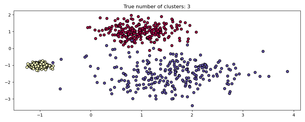
### Langkah 3: Membuat Dataset Sintetis
Dataset terdiri dari 3 buah cluster Gaussian.
```python
centers = [[1, 1], [-1, -1], [1.5, -1.5]]
X, labels_true = make_blobs(
n_samples=750, centers=centers, cluster_std=[0.4, 0.1, 0.75], random_state=0
)
plot(X, labels=labels_true, ground_truth=True)
```
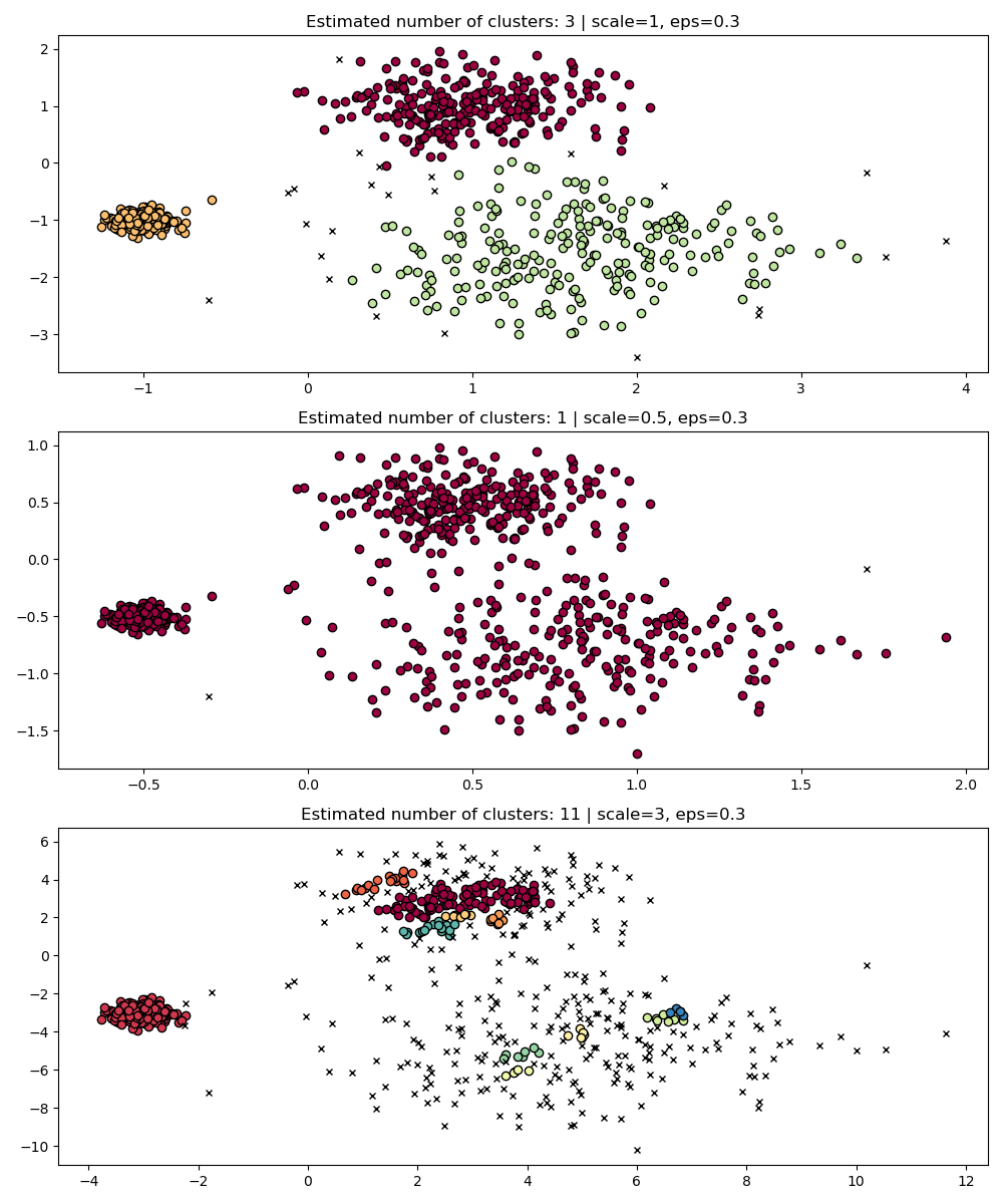
### Langkah 4: Uji *Scale Invariance* pada DBSCAN
Jalankan DBSCAN dengan `eps=0.3` pada dataset yang di-*scale*.
```python
fig, axes = plt.subplots(3, 1, figsize=(10, 12))
dbs = DBSCAN(eps=0.3)
for idx, scale in enumerate([1, 0.5, 3]):
dbs.fit(X * scale)
plot(X * scale, dbs.labels_, parameters={"scale": scale, "eps": 0.3}, ax=axes[idx])
```
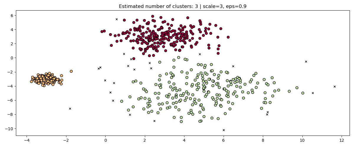
Perbaiki dengan mengubah `eps` sesuai skala:
```python
fig, axis = plt.subplots(1, 1, figsize=(12, 5))
dbs = DBSCAN(eps=0.9).fit(3 * X)
plot(3 * X, dbs.labels_, parameters={"scale": 3, "eps": 0.9}, ax=axis)
```
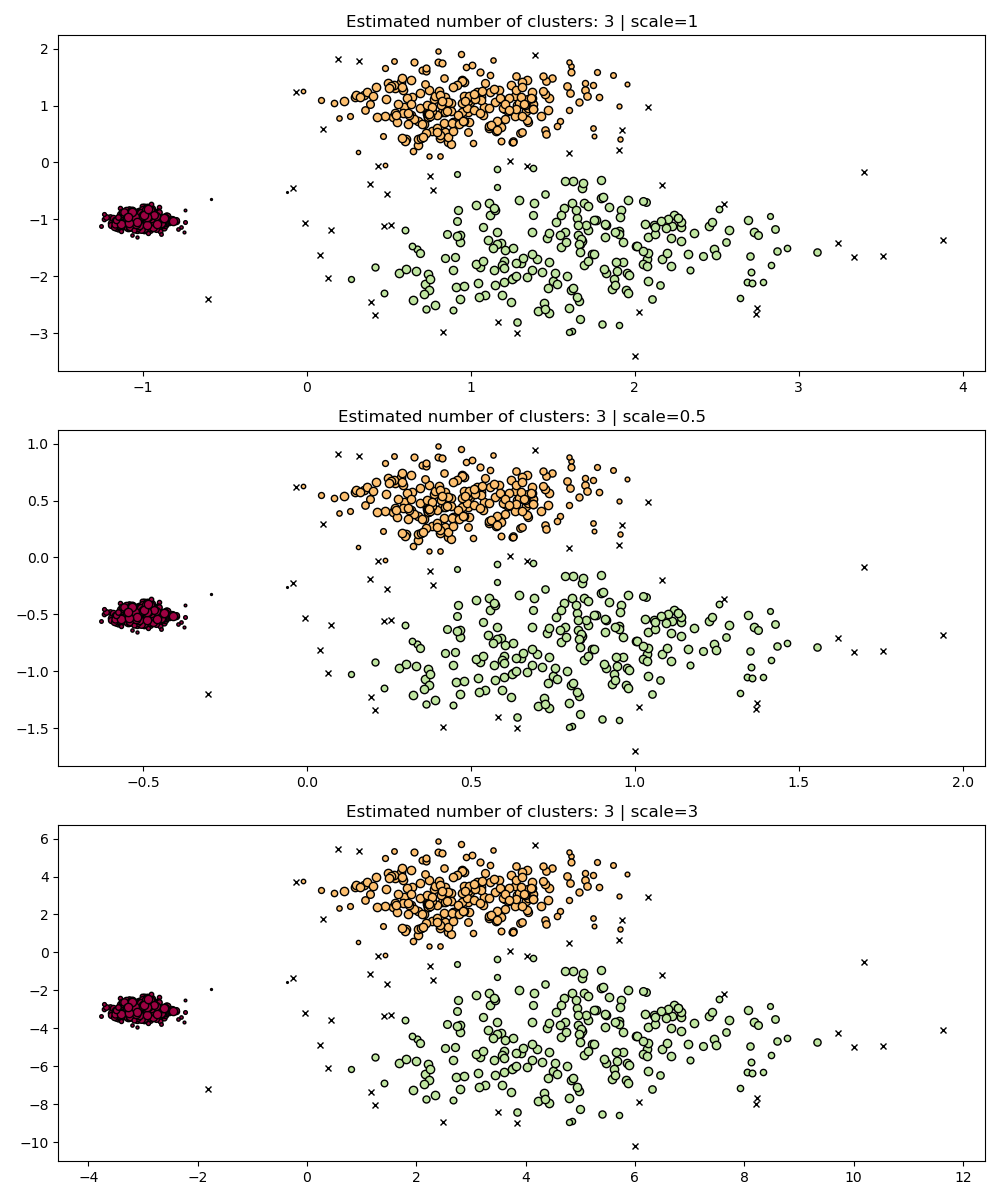
### Langkah 5: Bandingkan dengan HDBSCAN (lebih robust)
Jalankan HDBSCAN pada dataset berskala berbeda.
```python
fig, axes = plt.subplots(3, 1, figsize=(10, 12))
hdb = hdbscan.HDBSCAN()
for idx, scale in enumerate([1, 0.5, 3]):
hdb.fit(X * scale)
plot(X * scale, hdb.labels_, hdb.probabilities_, ax=axes[idx], parameters={"scale": scale})
```
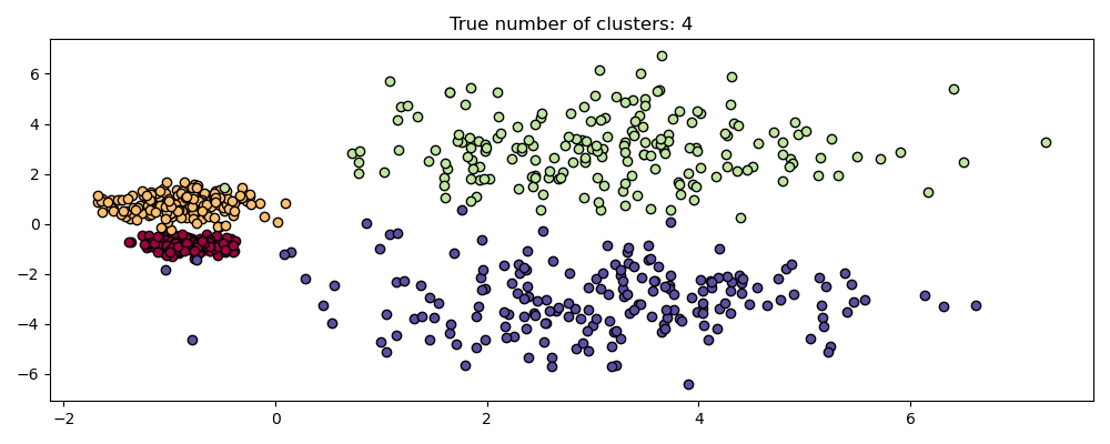
### Langkah 6: Multi-Scale Clustering
Buat dataset baru dengan kepadatan berbeda.
```python
centers = [[-0.85, -0.85], [-0.85, 0.85], [3, 3], [3, -3]]
X, labels_true = make_blobs(
n_samples=750, centers=centers, cluster_std=[0.2, 0.35, 1.35, 1.35], random_state=0
)
plot(X, labels=labels_true, ground_truth=True)
```
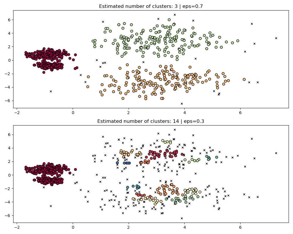
Bandingkan DBSCAN dengan `eps` berbeda:
```python
fig, axes = plt.subplots(2, 1, figsize=(10, 8))
params = {"eps": 0.7}
dbs = DBSCAN(**params).fit(X)
plot(X, dbs.labels_, parameters=params, ax=axes[0])
params = {"eps": 0.3}
dbs = DBSCAN(**params).fit(X)
plot(X, dbs.labels_, parameters=params, ax=axes[1])
```
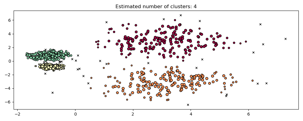
Jalankan HDBSCAN:
```python
hdb = hdbscan.HDBSCAN().fit(X)
plot(X, hdb.labels_, hdb.probabilities_)
```
###